The solution to any complex engineering problem involves generating multi-variable functions,constructing N-dimensional surfaces and, finally, applying powerful optimization software to find minima or maxima. Whether it’s designing bridges, integrated circuits or self-driving cars; modern engineers navigate complex mathematical surfaces while avoiding numerical black holes. In this blog post, I hope to give a brief introduction to the challenges involved and advice on how modern engineering software avoids these potentially fatal errors.
But first, a little math. Let’s revisit how multiplication maps a function in 1 dimension.
\[ y = \alpha x \]
In a physical sense, multiplying \(x\) by \(\alpha\) to get \(y\) represents
Shrinking \(x\) when \(0 < \alpha < 1\)
Stretching \(x\) when \(\alpha > 1\)
Rotating \(x\) by 180 degrees when \(\alpha = -1\)
Rotating \(x\) by 0 degrees when \(\alpha = 1\)
Removing a dimension from \(x\) when \(\alpha = 0\). Once you multiply by zero, no amount of stretching, shrinking or rotating can reverse it.
Of course, you can apply these operations on top of each other by repeated multiplication. -5*x can be interpreted as stretching x by 5 and then rotating by 180 degrees. Division is just reversing these operations… except for the last one.
\[ y = \frac{x}{\alpha} = \alpha^{-1} x \]
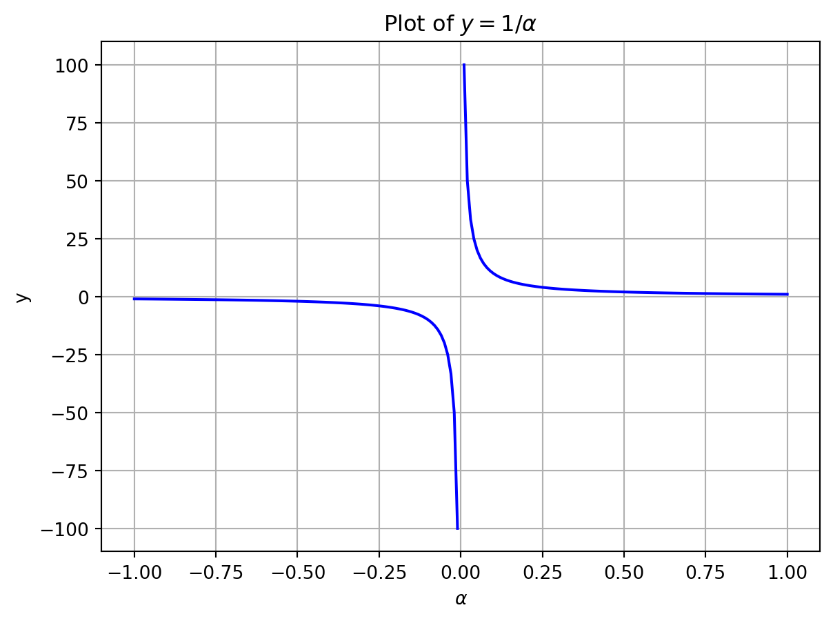
Remember that multiplying-by-zero removes a dimension. So how can we try to get it back? Let’s set \(x = 1\) and plot the values around \(\alpha = 0\) to see what this desperate struggle looks like.
Code
import numpy as npimport matplotlib.pyplot as pltdelta =0.01left_limit =-1right_limit =1# plot negative half of real number linex_left = np.arange(left_limit, 0, delta)plt.plot(x_left, 1.0/ x_left, "b")# plot positive half of real number linex_right = np.arange(delta, right_limit+delta, delta)plt.plot(x_right, 1.0/ x_right, "b")plt.title(r'Plot of $y = 1/\alpha$')plt.xlabel(r'$\alpha$')plt.ylabel("y")plt.grid(True)plt.show()
Figure 1: Plot on the real number line. A singularity clearly exists at x = 0.
Depending on how you approach zero, \(y = 1/\alpha\) tends towards \(+\infty\) or \(-\infty\). So should \(y\) be positive or negative at \(\alpha=0\)? We really can’t answer this, so it is best to say that division is undefined at \(\alpha = 0\). We cannot add back a dimension that has already been lost.
Now let’s look at 2 dimensions. We want to be able to stretch, shrink and rotate a point in space the same way we could with 1-D multiplication.
Matrix Multiplication is a useful tool that can do all of these things in higher dimensions. The notation is similar but we use a bold x and a capital, italicized A with the same shorthand as the 1-D case: \[
\mathbf{y} = A\mathbf{x}
\]
In 2 dimensions, we can visualize x as an arrow with x and y coordinates. The 2-D matrix \(A\) is a bit more abstract; it is defined a 2-by-2 tile of 4 numbers: \(a, b, c\) and \(d\):
\[A \mathbf{x} =
\begin{bmatrix}a & b \\ c & d\end{bmatrix}
\]
and matrix multiplication is defined as multiply and adding the rows of \(A\) to the (x,y) coordinates of x. \[
A \mathbf{x} =
\begin{bmatrix}a & b \\ c & d\end{bmatrix}
\begin{bmatrix}x \\ y \end{bmatrix}=\begin{bmatrix} a x + b y \\ c x + d y \end{bmatrix}
\]
To stretch and shrink in 2 dimensions, we use a diagonal matrix \[
\begin{bmatrix}\alpha & 0 \\ 0 & \beta\end{bmatrix}
\begin{bmatrix}x \\ y \end{bmatrix}=\begin{bmatrix} \alpha x \\ \beta y \end{bmatrix}
\]
To rotate by an angle \(\theta\) we can multiply by a rotation matrix
\[
\begin{bmatrix}\cos(\theta)& -\sin(\theta)\\ \sin(\theta) & \cos(\theta)\end{bmatrix}
\begin{bmatrix}x \\ y \end{bmatrix}=\begin{bmatrix} \cos(\theta) x - \sin(\theta) y \\ \sin(\theta) x + \cos(\theta) y \end{bmatrix}
\]
But what about losing a dimension like the 1 dimensional case? We can find it hiding in the reverse process. The inverse of a matrix multiplication reverses the process in the same way 1-D division does. \[
A^{-1}(A \mathbf{x}) =
\frac{1}{ad - bc}\begin{bmatrix}
d & -b \\ -c & a
\end{bmatrix}\left(
\begin{bmatrix} a x + b y \\ c x + d y \end{bmatrix}
\right)
= \begin{bmatrix} x \\ y \end{bmatrix}
\]
It now becomes obvious that we lose dimension(s) when \(ad - bc = 0\).
So how is this relevant to our everyday life?
In engineering, we start with a series of (usually complicated) equations that model some sort of desired behavior. Solving these equations tells us if our bridge will stay standing, our smartphone works correctly or if our self-driving car will stay on the road.
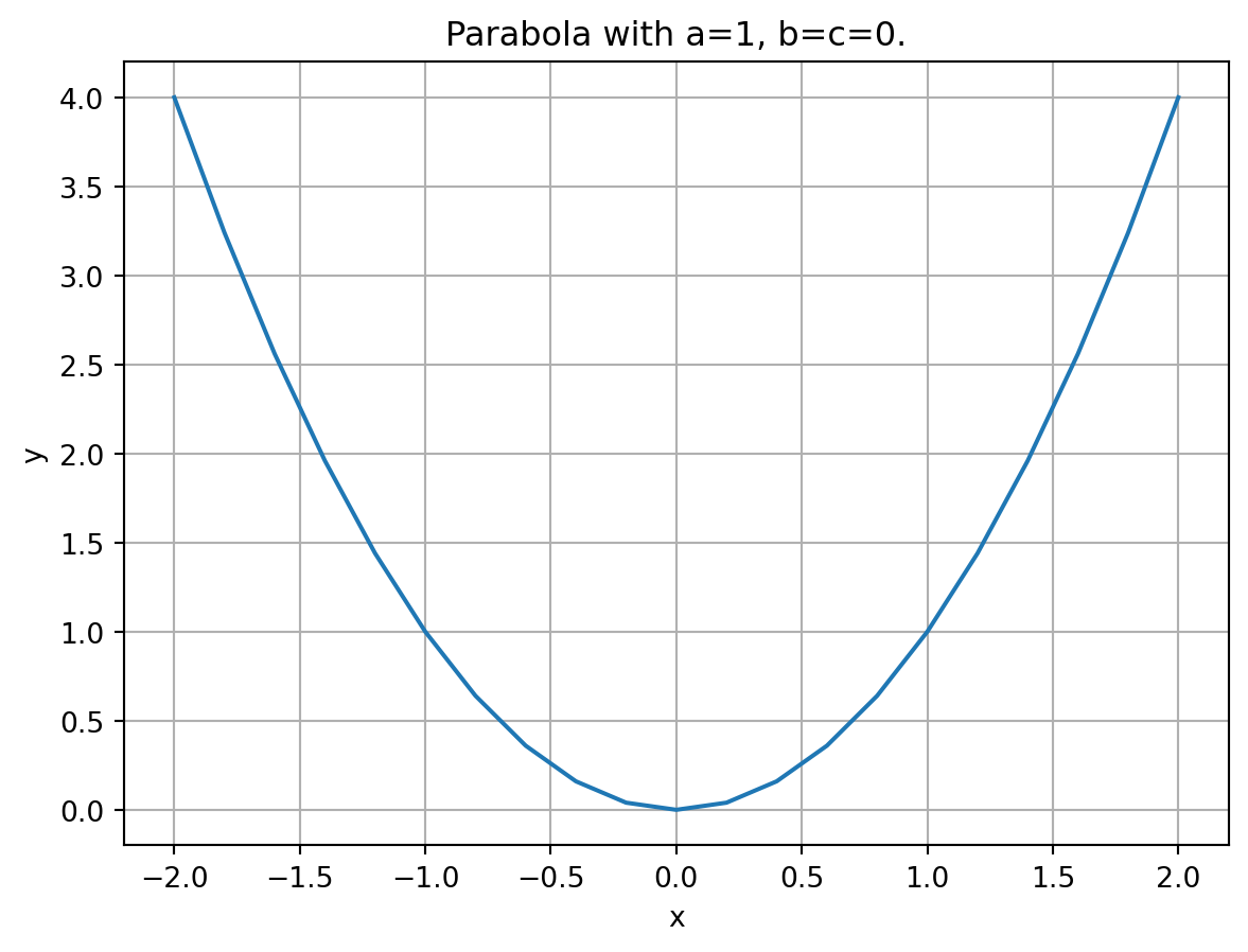
When trying to solve a complicated system of equations, engineers try to approximate everything as the simplest possible shapes: lines and parabolas. We’ve all seen these in grade school: \(y = ax^2 + bx + c\).
Code
import numpy as npimport matplotlib.pyplot as plttotal_points =21bounding_box =2x = np.linspace(-bounding_box, bounding_box, total_points)quadratic =lambda x,a,b,c: (a*x + b)*x + ca =1b =0c =0plt.plot(x, quadratic(x, a, b, c))plt.xlabel('x')plt.ylabel('y')plt.title('Parabola with a=1, b=c=0.')plt.grid(True)plt.show()
Figure 2: Positive definite quadratic function. Has a single, lowest point.
In 2 dimensions, this can be represented as a symmetric matrix where \(b = c\)
\[
A = \begin{bmatrix}a & b \\ b & d\end{bmatrix}, \quad \text{and }
A^{-1} = \frac{1}{ad-b^2}\begin{bmatrix}d & -b \\ -b & a\end{bmatrix}
\]
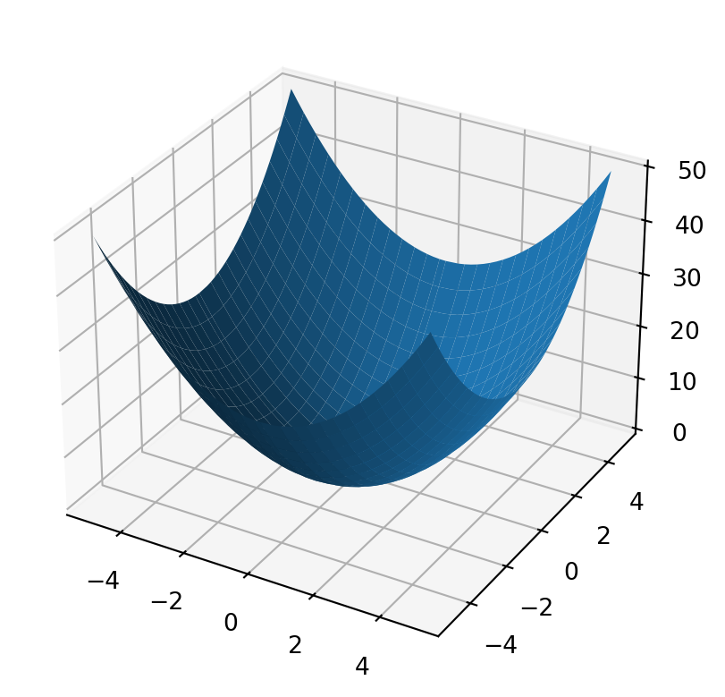
In higher dimensions there are 3 important types of parabolas: positive definite, negative definite and indefinite.
Code
import numpy as npimport matplotlib.pyplot as pltN =51bound =5grid_width2d = np.linspace(-bound, bound, N)grid_width2d[int(N/2)+1] =0x, y = np.meshgrid(grid_width2d, grid_width2d)quadratic =lambda x,y,a,b,c: a * np.multiply(x,x) +2*b*np.multiply(x, y) + c * np.multiply(y, y)fig, ax = plt.subplots( subplot_kw={"projection": "3d"} )ax.plot_surface(x, y, quadratic(x, y, 1.0, 0, 1))plt.show()
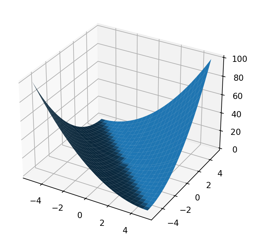
Figure 3: Positive definite quadratic function. Has a single, lowest point. These types of problems are common in controlling robots or self-driving cars.
Code
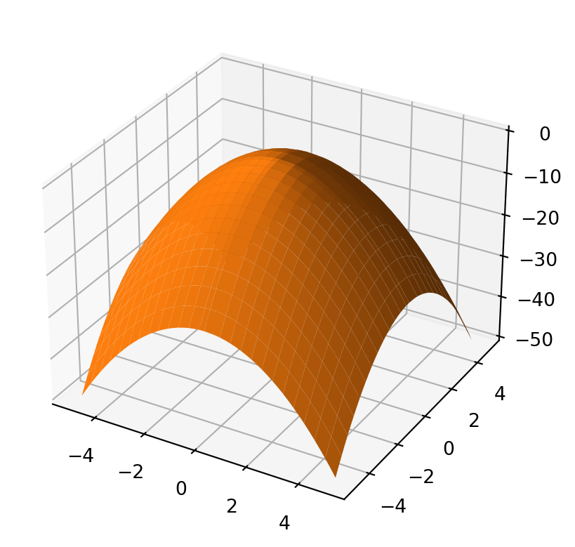
import numpy as npimport matplotlib.pyplot as pltfrom matplotlib.colors import TABLEAU_COLORSN =51bound =5grid_width2d = np.linspace(-bound, bound, N)grid_width2d[int(N/2)+1] =0x, y = np.meshgrid(grid_width2d, grid_width2d)quadratic =lambda x,y,a,b,c: a * np.multiply(x,x) +2*b*np.multiply(x, y) + c * np.multiply(y, y)fig, ax = plt.subplots( subplot_kw={"projection": "3d"} )ax.plot_surface(x, y, quadratic(x, y, -1.0, 0, -1.0), color=TABLEAU_COLORS['tab:orange'])plt.show()
Figure 4: Negative definite quadratic function. Has a single highest point. These types of curves are found in artificial intelligence models.
Code
import numpy as npimport matplotlib.pyplot as pltN =51bound =5grid_width2d = np.linspace(-bound, bound, N)grid_width2d[int(N/2)+1] =0x, y = np.meshgrid(grid_width2d, grid_width2d)quadratic =lambda x,y,a,b,c: a * np.multiply(x,x) +2*b*np.multiply(x, y) + c * np.multiply(y, y)fig, ax = plt.subplots( subplot_kw={"projection": "3d"} )ax.plot_surface(x, y, quadratic(x, y, -1.0, 0.0, 1.0), color=TABLEAU_COLORS['tab:green'])plt.show()
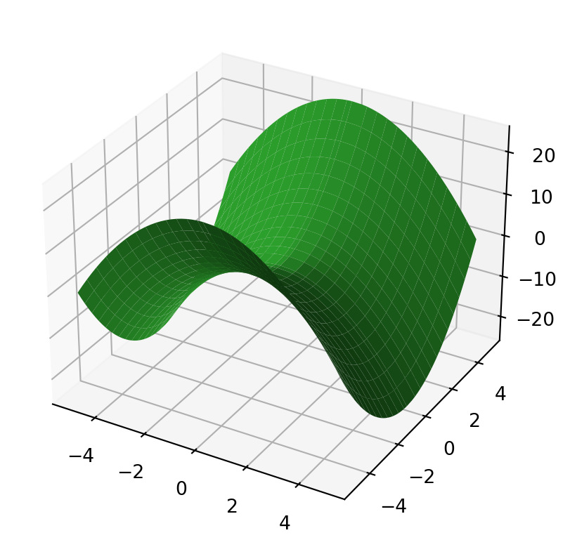
Figure 5: Indefinite quadratic function. Has no high or low points. Sometimes called a ‘Saddle Point’ curve because it looks like a horse saddle. These types of curves are found in resource scheduling problems – like how online shipping or power distribution are implemented.
When optimizing over an engineering model, the software is constantly updating its “understanding” of the terrain by adjusting the \(a\), \(b\) and \(d\) values. It then uses the inverse, \(A^{-1}\) to move along the surface. When each of these shapes are encountered, a different strategy is needed if you’re seeking the lowest or highest point (an optimal design). This is how optimization software fundamentally works.
But what happens if our software approximates our model where \(ad - b^2 = 0\)? The inverse \(A^{-1}\) involves division by zero and no progress can be made. This is uncommon, but by no means is it rare. It can cause a system to freeze up and needs to be accounted for. Let’s look at one such case where \(a = b = d = 1\).
Code
import numpy as npimport matplotlib.pyplot as pltN =51bound =5grid_width2d = np.linspace(-bound, bound, N)grid_width2d[int(N/2)+1] =0x, y = np.meshgrid(grid_width2d, grid_width2d)quadratic =lambda x,y,a,b,d: a * np.multiply(x,x) +2*b*np.multiply(x, y) + d * np.multiply(y, y)fig, ax = plt.subplots( subplot_kw={"projection": "3d"} )b =1.0d =1.0a =1.0assert(abs(a*d - d**2) <1e-12)ax.plot_surface(x, y, quadratic(x, y, a, b, d))plt.show()
Figure 6: Positive semi-definite quadratic function. Has infinitely many lowest points.
If you were to stand at the base of the this curve, you would see infinite repetition down the middle. In our black hole analogy, this is sort of like hovering around the photonsphere where light can theoretically stay in orbit. If you were to look in this direction, you would see the back of your head. If you look slightly off-center, you would see many repeating images of the back of your head.
Higher dimensional division-by-zero. Everything repeats forever in that direction.
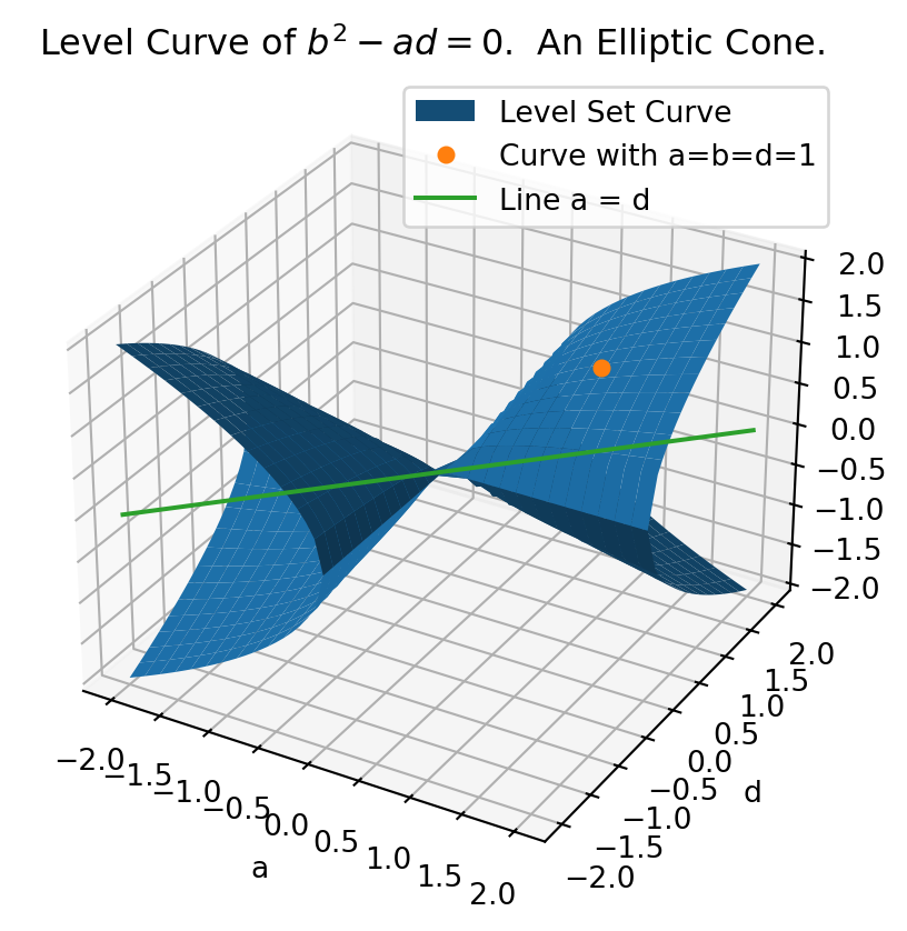
This is where state-of-the-art optimization software can intervene and prevent system failure. This software will recognize how these curves warp near the cone \(ad - b^2 = 0\). Each point on this curve represents a terrain like in Figure 6.
Code
import numpy as npimport matplotlib.pyplot as pltfrom matplotlib.colors import TABLEAU_COLORS# plot ad - b^2 = 0fig, ax = plt.subplots( subplot_kw={"projection": "3d"} )# Keep this an odd number to avoid graphical issue.N =51bound =2grid_width2d = np.linspace(-bound, bound, N)grid_width2d[int(N/2)+1] =0A2d, D2d = np.meshgrid(grid_width2d, grid_width2d)multiply = np.multiply(A2d, D2d)multiply[multiply <0] = np.nan # ignore negative values, no value of "b" can make these zero.B_zero_pos = np.sqrt(multiply)B_zero_neg =-np.sqrt(multiply)ax.plot_surface(A2d, D2d, B_zero_pos, zorder=10, label="Level Set Curve")ax.plot_surface(A2d, D2d, B_zero_neg, color = TABLEAU_COLORS['tab:blue'], zorder=20)a =1b =1d =1ax.plot(a, b, d, color=TABLEAU_COLORS['tab:orange'], zorder=30, markersize=5, lw=0, marker='o', label='Curve with a=b=d=1')ax.plot( grid_width2d, grid_width2d, np.zeros((1, N)), label="Line a = d", zorder=30, color=TABLEAU_COLORS['tab:green'],)# Label everything.ax.legend()ax.set_xlabel("a")ax.set_ylabel("d")ax.set_zlabel("b")ax.set_title(r'Level Curve of $b^2 - ad = 0$. An Elliptic Cone.')plt.grid(True)plt.show()
Figure 7: Level Set Curve where \(ad - b^2 = 0\). Every point represents a 2-D parabola that repeats itself in one or more directions. At the origin (0,0) we have \(a = b = c = 0\) where every direction repeats itself.
This shape helps inform us of several strategies to “push away” from this cone if we ever find ourselves near it. The simplest way to do this is by moving parallel to the green line . This just means choosing a \(\Delta\) such that \((a+\Delta)(d + \Delta) - b^2 \neq 0\). Setting \(\Delta \geq |b|\) is a common strategy that moves us safely away from this cone. If \(b \approx 0\), then setting \(\Delta = 1\) is a decent fallback.
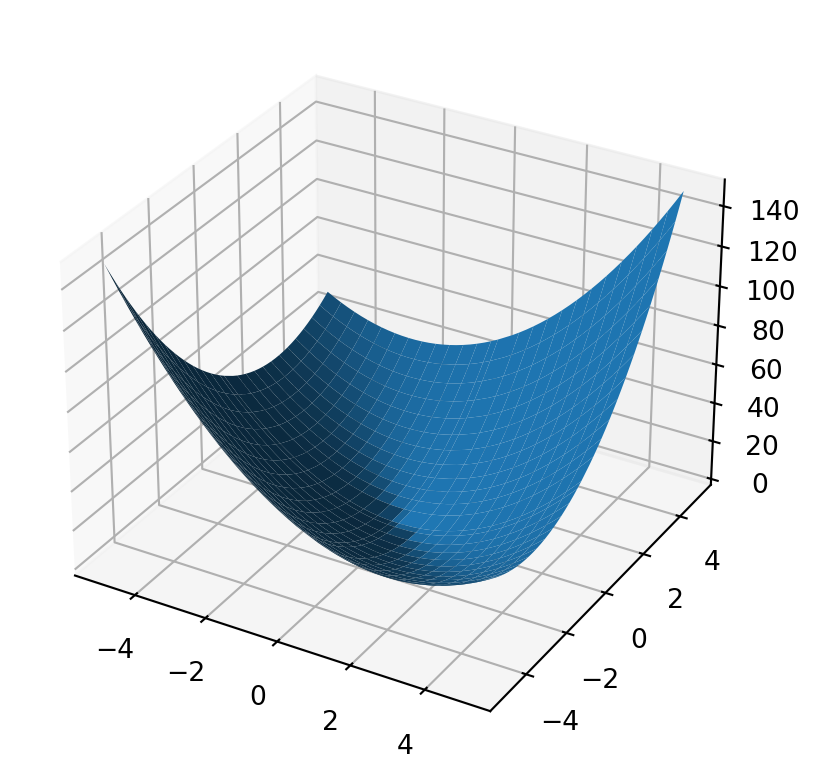
In the case of Figure 6, our updated model would look like the following:
Code
import numpy as npimport matplotlib.pyplot as pltN =51bound =5grid_width2d = np.linspace(-bound, bound, N)grid_width2d[int(N/2)+1] =0x, y = np.meshgrid(grid_width2d, grid_width2d)quadratic =lambda x,y,a,b,d: a * np.multiply(x,x) +2*b*np.multiply(x, y) + d * np.multiply(y, y)fig, ax = plt.subplots( subplot_kw={"projection": "3d"} )a =2b =1d =2ax.plot_surface(x, y, quadratic(x, y,a, b, d))plt.show()
Figure 8: Semi-definite curve now becomes positive definite with a single lowest point.
This model curve now contains a practical minimum value that can prevent system failure.
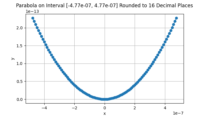
In the real world, the problem state above doesn’t just happen when \(ad - b^2 = 0\). Every computer has rounding error that increases as the numbers get larger – or the divisor gets smaller. Rounding errors on a 64-bit computer processor become destructive when \(|ad - b^2| < 2^{-26} \approx 1.48 \cdot 10^{-8}\). Beyond this bound, anything you do will increasingly destabilize the behavior of your program. In addition, hardware constraints mean that if \(|ad - b^2| < 2^{-52} \approx 2.22 \cdot 10^{-16}\), your software will behave randomly and there is no hope of making any sense of your program’s behavior. The animation below shows this effect on a 1-D parabola as \(x\) approaches \(2^{-26}\). Note how the shape breaks down. You have entered a numerical black hole. Again, state-of-the-art optimization software can recognize and prevent these problems.
Parabola rounded to 16 digits of precision. As the interval gets smaller towards ~1.48e-8, we see the effects of rounding error.
In summary, modern engineering software fails when we cannot find an absolute minimum or maximum, try to divide near zero and go beyond rounding error guidelines. Therefore, to prevent system-wide failures, I recommend all engineering software should be monitored by state-of-the-art optimization software which can not only optimize efficiency but also recognize and prevent these problems before they happen. It is especially critical that the engineering and optimization programs communicate synergistically in real time. This can prevent power networks from failing, autonomous cars from crashing and allow drones to complete their missions.
If you are interested in learning more about this technology and its uses, please contact support@ribbonopt.com for more information. We would love to understand what kinds of issues you are facing and how our tools can better serve your engineering staff.